Machine Learning Part 5: How we evaluate classification algorithms
import matplotlib.pyplot as plt
import matplotlib
import numpy as np
import pandas as pd
from sklearn import datasets
matplotlib.rcParams['figure.figsize'] = [20, 10]
In this note we would like to explain two concepts
- What classification is
- What Logistic Regression is.
- And finally, probably the most complicated here: How to evaluate classification.
Classification problem
Classification problem is a kind of supervised Machine Learning Algorithm whose target are set of discrete values (classes).
There few kinds of classifications.
- Binary classification: when an observation can belong to just one of two classes. Here often there is just one class and we try to determine if an observation belongs to it or not.
- Multiclass classification: when an observation can be belong to just one of many classes.
- Multilabel classification: When an observation can belong to zero or many classes.
Example
We would like to predict if a patient is sick or not based on her/his blood test. This is classification problem. Moreover, since we have just two classes it is also called binary classification.
Example
We would like to say if a given photo contains a hot dog. This is also binary classification.
Example
We would like tell what is on a given photo. For example ImageNet is a large dataset with images with that have object of thousands of different classes. This a an example of multiclass classification. If one image can have more than one object we deal with multilabel classification.
Logistic Regression
Logistic Regression, although called regression, is a binary classification algorithm. Why is it called regression? It is because, the output of this algorithm is a probability, so it is a continuous number between zero and one. Let’s look at example. Imagine that we would like to predict if a image contains a hot dog. So here we have to classes: first class hot dog contains images with a hot dog and the other not a hot dog, images that do not contain a hot dog. So we can label by 1 the first class and by 0 the second. Then the output of the logistic regression algorithm is a probability of having a hot dog on a image. That is, if the output is 0.9 we are likely to see hot dog. On the other hand if the output in 0.03 than we are very likely to have an image without a hot dog.
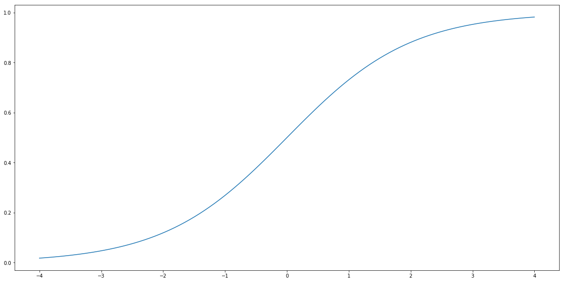
So how we fit probabilities, that are numbers between zero and one into linear regression that produce output being unbounded real number? We use a function called sigmoid. This function is denoted by $\sigma$ and is defined by the formula:
\[\sigma(t) = \frac{1}{1+\exp(-t)}.\]Let’s plot it.
def sigmoid(t):
    return 1/(1+np.exp(-t))

t = np.linspace(-4, 4, 100)
plt.plot(t, sigmoid(t))

plt.show()
Logistic Regression is a method that tries to find $a$ and $b$ such that $\hat{Y}$ given by the formula
\[\hat{Y} = \sigma(a X + b) = \frac{1}{1+\exp(a X + b)}\]gives the best possible probabilities that $X$ belongs of not to the class labeled by 1.
Let’s see how it works with an example.
Dataset
Here we will study data extracted from images of a breast mass. We are going to predict if a tumor observed there is malignant or not. First we will try to address the following problem.
Question Can we build a model that based on the radius of a tumor can classify if the tumor is malignant or not?
For that let’s load our data.
from sklearn.datasets import load_breast_cancer
data = load_breast_cancer()
list(data.target_names)
['malignant', 'benign']
print(data.DESCR)
.. _breast_cancer_dataset:

Breast cancer wisconsin (diagnostic) dataset
--------------------------------------------

**Data Set Characteristics:**

    :Number of Instances: 569

    :Number of Attributes: 30 numeric, predictive attributes and the class

    :Attribute Information:
        - radius (mean of distances from center to points on the perimeter)
        - texture (standard deviation of gray-scale values)
        - perimeter
        - area
        - smoothness (local variation in radius lengths)
        - compactness (perimeter^2 / area - 1.0)
        - concavity (severity of concave portions of the contour)
        - concave points (number of concave portions of the contour)
        - symmetry
        - fractal dimension ("coastline approximation" - 1)

        The mean, standard error, and "worst" or largest (mean of the three
        largest values) of these features were computed for each image,
        resulting in 30 features.  For instance, field 3 is Mean Radius, field
        13 is Radius SE, field 23 is Worst Radius.

        - class:
                - WDBC-Malignant
                - WDBC-Benign

    :Summary Statistics:

    ===================================== ====== ======
                                           Min    Max
    ===================================== ====== ======
    radius (mean):                        6.981  28.11
    texture (mean):                       9.71   39.28
    perimeter (mean):                     43.79  188.5
    area (mean):                          143.5  2501.0
    smoothness (mean):                    0.053  0.163
    compactness (mean):                   0.019  0.345
    concavity (mean):                     0.0    0.427
    concave points (mean):                0.0    0.201
    symmetry (mean):                      0.106  0.304
    fractal dimension (mean):             0.05   0.097
    radius (standard error):              0.112  2.873
    texture (standard error):             0.36   4.885
    perimeter (standard error):           0.757  21.98
    area (standard error):                6.802  542.2
    smoothness (standard error):          0.002  0.031
    compactness (standard error):         0.002  0.135
    concavity (standard error):           0.0    0.396
    concave points (standard error):      0.0    0.053
    symmetry (standard error):            0.008  0.079
    fractal dimension (standard error):   0.001  0.03
    radius (worst):                       7.93   36.04
    texture (worst):                      12.02  49.54
    perimeter (worst):                    50.41  251.2
    area (worst):                         185.2  4254.0
    smoothness (worst):                   0.071  0.223
    compactness (worst):                  0.027  1.058
    concavity (worst):                    0.0    1.252
    concave points (worst):               0.0    0.291
    symmetry (worst):                     0.156  0.664
    fractal dimension (worst):            0.055  0.208
    ===================================== ====== ======

    :Missing Attribute Values: None

    :Class Distribution: 212 - Malignant, 357 - Benign

    :Creator:  Dr. William H. Wolberg, W. Nick Street, Olvi L. Mangasarian

    :Donor: Nick Street

    :Date: November, 1995

This is a copy of UCI ML Breast Cancer Wisconsin (Diagnostic) datasets.
https://goo.gl/U2Uwz2

Features are computed from a digitized image of a fine needle
aspirate (FNA) of a breast mass.  They describe
characteristics of the cell nuclei present in the image.

Separating plane described above was obtained using
Multisurface Method-Tree (MSM-T) [K. P. Bennett, "Decision Tree
Construction Via Linear Programming." Proceedings of the 4th
Midwest Artificial Intelligence and Cognitive Science Society,
pp. 97-101, 1992], a classification method which uses linear
programming to construct a decision tree.  Relevant features
were selected using an exhaustive search in the space of 1-4
features and 1-3 separating planes.

The actual linear program used to obtain the separating plane
in the 3-dimensional space is that described in:
[K. P. Bennett and O. L. Mangasarian: "Robust Linear
Programming Discrimination of Two Linearly Inseparable Sets",
Optimization Methods and Software 1, 1992, 23-34].

This database is also available through the UW CS ftp server:

ftp ftp.cs.wisc.edu
cd math-prog/cpo-dataset/machine-learn/WDBC/

.. topic:: References

   - W.N. Street, W.H. Wolberg and O.L. Mangasarian. Nuclear feature extraction
     for breast tumor diagnosis. IS&T/SPIE 1993 International Symposium on
     Electronic Imaging: Science and Technology, volume 1905, pages 861-870,
     San Jose, CA, 1993.
   - O.L. Mangasarian, W.N. Street and W.H. Wolberg. Breast cancer diagnosis and
     prognosis via linear programming. Operations Research, 43(4), pages 570-577,
     July-August 1995.
   - W.H. Wolberg, W.N. Street, and O.L. Mangasarian. Machine learning techniques
     to diagnose breast cancer from fine-needle aspirates. Cancer Letters 77 (1994)
     163-171.
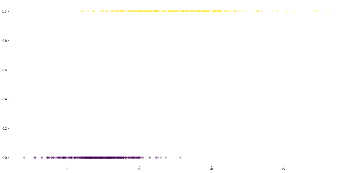
So if target is 1 the tumor is malignant. Otherwise, if the target is 0, the tumor is benign.
y = data.target == 0 # if zero then we detect malignant tumor.

plt.scatter(data.data[:, [0]], y, alpha=0.3, c=y)
plt.show()
# 1. Prepare data
X = data.data[:, [0]] # only one column, radius
y = data.target == 0

# 2. Split data into train and test.
from sklearn.model_selection import train_test_split
X_train, X_test, y_train, y_test = train_test_split(X, y, test_size=0.3, random_state=666)

# 3. Build a model
from sklearn.linear_model import LogisticRegression
clf = LogisticRegression()

# 4. Fit model to train data.
clf.fit(X_train, y_train)

# 5. Caluate prediction on test set
y_test_hat = clf.predict(X_test)
/home/bartek/Envs/py3.6/lib/python3.6/site-packages/sklearn/linear_model/logistic.py:433: FutureWarning: Default solver will be changed to 'lbfgs' in 0.22. Specify a solver to silence this warning.
  FutureWarning)
Before we get to evaluation we need to discuss how we are evaluate if classification models. Let us explain then few concepts:
- accuracy,
- confusion matrix,
- precision and recall.
Evaluation 1: Accuracy
One way of evaluating a classification model is to calculate what percentage of classes we have predicted accurately.
n_sample = len(y_test)
correct_prediction = sum(y_test == y_test_hat)

# Accuracy
correct_prediction/n_sample
0.9122807017543859
90%! not bad.
The package sklearn has also convenient function that calculate accuracy score.
from sklearn.metrics import accuracy_score
accuracy_score(y_test, y_test_hat)
0.9122807017543859
We have said that the output of our model is not 1 or 0, that is if the observation is respectively malignant or not malignant tumor. Our real output is a probability that the observation is malignant. So we have to choose with which probability it implies that the tumor is malignant. The package sklearn does it for us and choose 50%. Hence output y_test_hat is already True or False.
However we can get also the probabilities. We can get them in sklearn using predict_prob method. It returns two columns, first is the probability of belonging to class 0 (benign cancer) and the second is the probability of belonging to class 1 (malignant cancer). They of course sum up to 1 and we only need the second column.
y_test_proba = clf.predict_proba(X_test)[:, 1]
y_test_prediction = y_test_proba >= 0.5
correct_prediction = sum(y_test == y_test_prediction)

# Accuracy
correct_prediction/n_sample
0.9122807017543859
Later when we discuss recall and precision, we will discuss when we choose 50% as a threshold for the decision and when not.
Evaluation 2: Confusion matrix
Imagine that in our dataset there is only 5% of observation with malignant tumor. Then one can get 95% accuracy just by labeling all observations as benign. Is it a good model? Not at all.
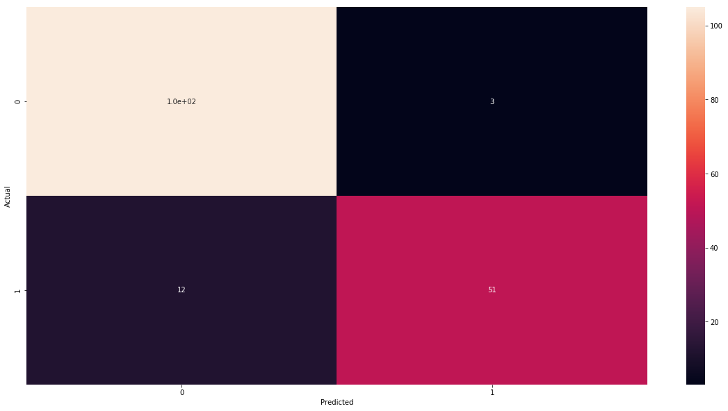
One can address this problem using confusion matrix. Confusion matrix matrix shows us complete picture how many images were correctly and incorrectly classified. As columns we put what is actual class of the observation and on rows what we have predicted. The easiest way of understanding it is to look at our example.
true_positive = sum(y_test & y_test_prediction)
false_positive = sum(~y_test & y_test_prediction)
true_negative = sum(~y_test & ~y_test_prediction)
false_negative = sum(y_test & ~y_test_prediction)

pd.DataFrame({
        "Predicted 0": [true_negative, false_negative],
        "Predicted 1": [false_positive, true_positive]
    },
    index= ["Actual 0", "Actual 1"]
)
| Predicted 0 | Predicted 1 | |
|---|---|---|
| Actual 0 | 105 | 3 |
| Actual 1 | 12 | 51 |
So we see that with respect to observations that were in class 0 (benign cancer) we have correctly classified 105 of them and 12 we have misclassified as malignant. And in the case on malignant observation we have 51 corrected predictions and 5 incorrect.
Again, there is a convenient function in sklearn that can do it for us.
from sklearn.metrics import confusion_matrix
cm = confusion_matrix(y_test, y_test_hat)
cm
array([[105,   3],
       [ 12,  51]])
One can get accuracy from confusion matrix by summing the number in the diagonal and then dividing it by the sum of all elements in the matrix.
cm.diagonal().sum()/cm.sum()
0.9122807017543859
Finally, we will transform cm into pandas.DataFrame and nicely plot using function heatmap from package seaborn.
import seaborn as sns


def get_cm_df(cm):
    labels = [0, 1]
    cm_df = pd.DataFrame(cm, index=labels, columns=labels)
    cm_df.index.name = 'Actual'
    cm_df.columns.name = 'Predicted'
    return cm_df

cm_df = get_cm_df(cm)
cm_df
| Predicted | 0 | 1 |
|---|---|---|
| Actual | ||
| 0 | 105 | 3 |
| 1 | 12 | 51 |
sns.heatmap(cm_df, annot=cm)
plt.show()
Evaluation 3: Precision and recall
Confusion matrix is four number that shows the complete picture how our model works. We can simplify it a bit by two concepts: precision and recall. Precision (also called positive predictive value (PPV)) measures how well we did with predicted positive examples. So it is defined by
\[\mathrm{Precision} = \frac{\mathrm{True\ positives}}{\mathrm{True\ positives} + \mathrm{False\ positives}}\]And recall (also called sensitivity, hit rate, or true positive rate (TPR)) measures how well we did with actual positives. That is
\[\mathrm{Recall} = \frac{\mathrm{True\ positives}}{\mathrm{True\ positives} + \mathrm{False\ negatives}}\]So in our case we have the following.
precision = true_positive/(true_positive + false_positive)
recall = true_positive/(true_positive + false_negative)
precision, recall
(0.9444444444444444, 0.8095238095238095)
Again we have convenient functions for calculating it.
from sklearn.metrics import precision_score, recall_score

precision_score(y_test, y_test_hat), recall_score(y_test, y_test_hat)
(0.9444444444444444, 0.8095238095238095)
Precision-recall trade-off
The best models have both precision and recall high. However, in general it is difficult to have both. But from a business perspective it sometimes important to focus on one of them. Moreover, often we can increase one and sacrifice the other. We will see how we can do this with Logistic Regression model. But before let me illustrate the problem with two examples.
Example
Imagine that we work for on-line shop. We are building a model that detects if a customer is unhappy. When we detect it, we would like to send them a coupon for 20 Eur to be spend in out shop. Of course we do not want to sent it to many users only to that we are sure that they are unhappy. So here we need a model with high precision and we can sacrifice recall.
Example
Sometimes we rather prefer high recall. In the cancer detection, we would rather prefer to have benign tumor misclassified and then do some extra exams to confirm that, than malignant cancer misclassified and having a patient dead during next few years.
In the case of Logistic Regression we can easily improve one of precision or recall by playing with threshold. Let me show it.
First we set a decision threshold to 75% and see how precision and recall have changed.
def precision_recall(y_true, y_proba, threshold):
    y_hat = y_proba >= threshold
    precision = 1 if sum(y_hat) == 0 else precision_score(y_true, y_hat) # we set precision to 1 if
                                                                         # there is no ones, this is a bit
                                                                         # techincal so do not worry
    return precision, recall_score(y_true, y_hat)

precision_recall(y_test, y_test_proba, .75)
(0.9714285714285714, 0.5396825396825397)
As you can see now we have increased the precision to 97% and the recall has dropped 54%. Let’s look also at confusion matrix.
def cm_matrix_from_threshold(y_true, y_proba, threshold):
    y_hat = y_proba >= threshold
    return confusion_matrix(y_true, y_hat)


get_cm_df(cm_matrix_from_threshold(y_test, y_test_proba, .75))
| Predicted | 0 | 1 |
|---|---|---|
| Actual | ||
| 0 | 107 | 1 |
| 1 | 29 | 34 |
So now we have only 35 observation predicted as malignant (before was 54), but only one is misclassified (before was 3). The cost of this is that we have more observation classified as saved (benign) and much more of them misclassified.
Now we set a decision threshold to 25%.
precision_recall(y_test, y_test_proba, .25)
(0.5504587155963303, 0.9523809523809523)
We see that precision has dropped to 55% but now recall is high 95%.
So let’s look at confusion matrix in order to find out why.
get_cm_df(cm_matrix_from_threshold(y_test, y_test_proba, .25))
| Predicted | 0 | 1 |
|---|---|---|
| Actual | ||
| 0 | 59 | 49 |
| 1 | 3 | 60 |
As we see, now among 63 malignant observations we have only 3 misclassified.
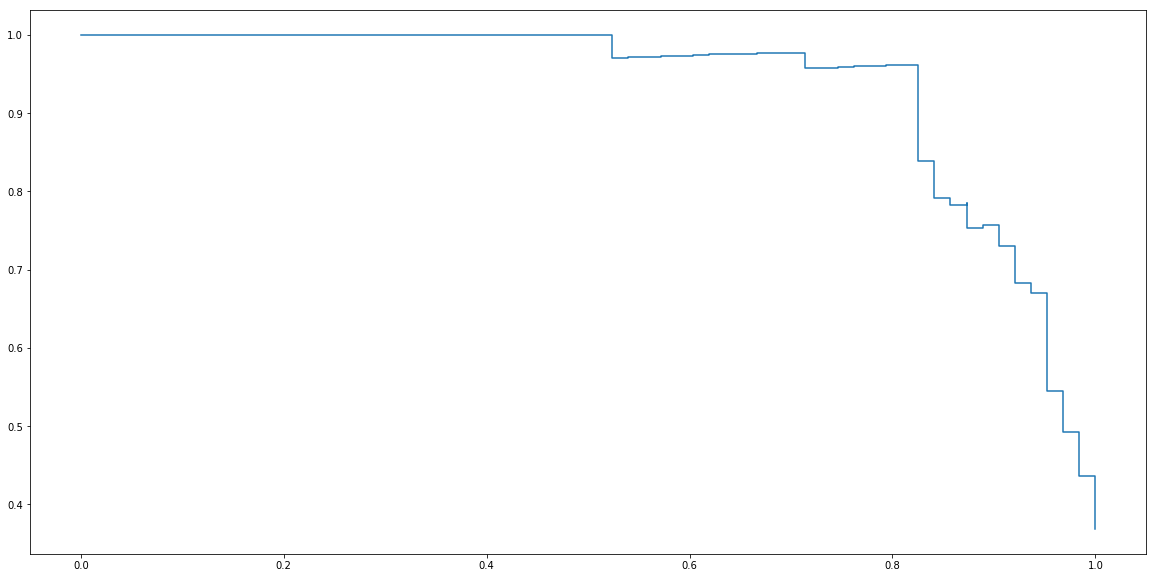
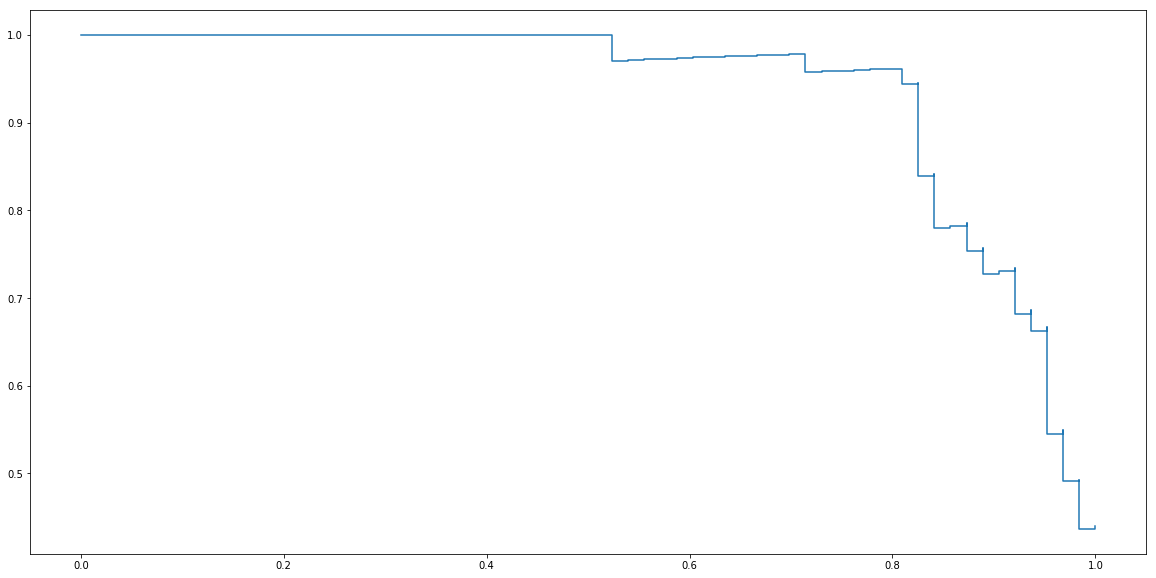
Finally, by varying threshold for zero to one and register corresponding precisions and recalls we can plot precision-recall curve.
ts = np.linspace(0, 1, 100)
precisions = []
recalls = []
for t in ts:
    p,r = precision_recall(y_test, y_test_proba, t)
    precisions.append(p)
    recalls.append(r)

plt.step(recalls, precisions)
plt.show()
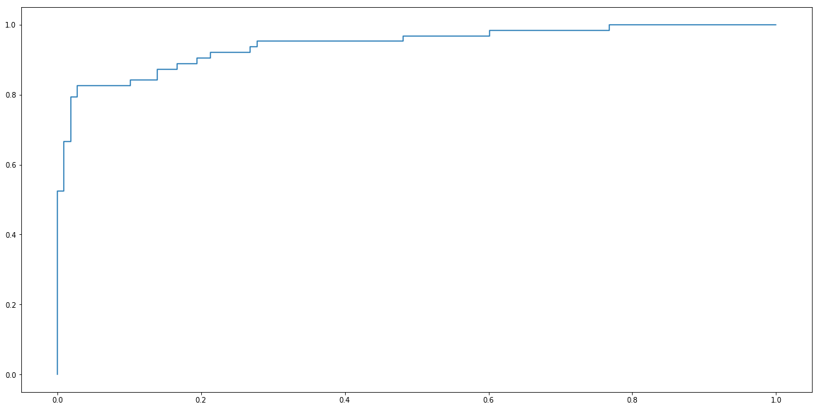
Package sklearn contains a function precision_recall_curve that calculate it for us. In order to use it, we need to provide y_score which are values of linear part of Logistic regression before applying sigmoid function. They can be obtained using decision_function method.
from sklearn.metrics import precision_recall_curve

y_test_score = clf.decision_function(X_test)
precisions, recalls, _ = precision_recall_curve(y_test, y_test_score)
plt.step(recalls, precisions)
plt.show()
Evaluation 4: F-score
As we said before, the best models have both precision and recall high. However, when it comes to compare models having two numbers can be difficult.
Example Imagine situation when one model has precision, recall respectively equal to 0.7, 0.65, and to 0.66, 0.69. So which one is better?
In this kind of situation it is useful to have just one simple criterion. And here it is common to use a metric called F-score.(or F1-score) This metric is defined by the following formula.
\[\mathrm{F-score} = \frac{2}{\frac{1}{\textrm{Precision}} + \frac{1}{\textrm{Recall}}}.\]Example-continuation So in our example we can compare precisions and recalls using F-score. Let’s do this.
def f_score(precision, recall):
    return 2/(1/precision + 1/recall)

f_score(0.7, 0.65), f_score(0.66, 0.69)
(0.674074074074074, 0.6746666666666666)
So the second one seems to be slightly better.
Now let’s come back to cancer example and calculate f-score for it.
f_score(precision_score(y_test, y_test_hat), recall_score(y_test, y_test_hat))
0.8717948717948718
Or using function form sklearn.
from sklearn.metrics import f1_score

f1_score(y_test, y_test_hat)
0.8717948717948718
Evaluation 5: AUC - Area under ROC curve
Let us finish with another very important evaluation. The problem is F-score is that, when we change threshold the F-score can also change. So what is a solution? One is to use the area under precision-recall curve we have seen before. And it is sometimes used. However, much more popular is the area under ROC curve. This metric is called AUC.
ROC curve
ROC curve is very similar to precision-recall curve, but instead of precision it uses false positive rate (FPR) also called fall-out. FPR is defined by the following formula.
\[\mathrm{FPR} = \frac{\mathrm{False\ positives}}{\mathrm{False\ positives} + \mathrm{True\ negatives} }\]def fpr(y_true, y_pred):
false_positive = sum(~y_true & y_pred)
true_negative = sum(~y_true & ~y_pred)
return false_positive/(false_positive + true_negative)
def fpr_recall(y_true, y_proba, threshold):
y_hat = y_proba >= threshold
fpr_score = fpr(y_true, y_hat)
return fpr_score, recall_score(y_true, y_hat)
ts = np.linspace(0, 1, 100)
fprs = []
recalls = []
for t in ts:
f,r = fpr_recall(y_test, y_test_proba, t)
fprs.append(f)
recalls.append(r)
plt.step(fprs, recalls)
plt.show()
Again, package sklearn contains convenient function for calculating ROC curve.
from sklearn.metrics import roc_curve

y_test_score = clf.decision_function(X_test)
fprs, recalls, _ = roc_curve(y_test, y_test_score)

plt.plot(fprs, recalls)
plt.fill_between(fprs, recalls, alpha=0.2, color='orange')
plt.show()
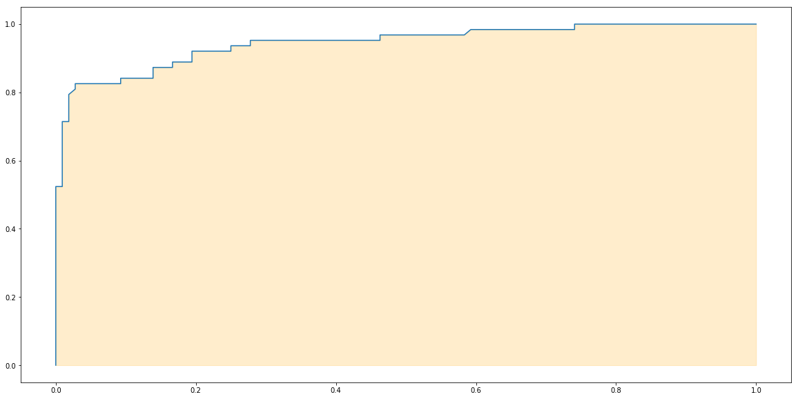
Finally the area under the ROC curve is AUC. Let’s use a function from sklearn to calculate it.
from sklearn.metrics import roc_auc_score

roc_auc_score(y_test, y_test_score)
0.9444444444444444
Extra There is also another curious way of calculating AUC. What we do we form all possible pairs of observation $(y_i, y_j)$ where $y_i$ is an negative observation (labeled with 0) and $y_j$ is a positive example (labeled with 1). Then we calculate if the scores (or probabilities) are in the right order, that is if the score of the observation i is lower than the score for the observation j. Then we calculate the fractions of corrected pairs to the all possible pair.
The following code implement it. And as you see the value is very close to the value given by roc_auc_score method from sklearn package.
total_count = 0
corrects = 0
for i in range(len(y_test)):
    if y_test[i] == 1:
        for j in range(len(y_test)):
            if y_test[j] == 0:
                total_count += 1
                if y_test_score[i] > y_test_score[j]:
                    corrects += 1

corrects/total_count
0.9442974720752498
Everything together
# 1. Prepare data
X = data.data[:, [0]]
y = data.target == 0

# 2. Split data into train and test.
from sklearn.model_selection import train_test_split
X_train, X_test, y_train, y_test = train_test_split(X, y, test_size=0.3, random_state=666)

# 3. Build a model
from sklearn.linear_model import LogisticRegression
clf = LogisticRegression()

# 4. Fit model to train data.
clf.fit(X_train, y_train)

# 5. Evaluate model on test data.
y_test_hat = clf.predict(X_test)
y_test_score = clf.decision_function(X_test)
print("AUC :", roc_auc_score(y_test, y_test_score))
print("F1-score :", f1_score(y_test, y_test_hat))
print("Precision :", precision_score(y_test, y_test_hat))
print("Recall :", recall_score(y_test, y_test_hat))
print("Accuracy score :", accuracy_score(y_test, y_test_hat))
AUC : 0.9444444444444444
F1-score : 0.8717948717948718
Precision : 0.9444444444444444
Recall : 0.8095238095238095
Accuracy score : 0.9122807017543859


/home/bartek/Envs/py3.6/lib/python3.6/site-packages/sklearn/linear_model/logistic.py:433: FutureWarning: Default solver will be changed to 'lbfgs' in 0.22. Specify a solver to silence this warning.
  FutureWarning)
Multiple Logistic Regression
Now we can easily generalize Logistic Regression with one exploratory variable to many variables the same way we can generalize Linear Regression to Multiple Linear Regression. So Multiple Logistic Regression is a model that have $n+1$ parameters $a_0$, $a_1$,… $a_n$ and $b$ and it is given by formula:
\[\hat{y} = \sigma(a_0x_0 + a_1x_1 + \ldots + a_nx_n + b) = \frac{1}{1+\exp(a_0x_0 + a_1x_1 + \ldots + a_nx_n + b)}.\]Actually the code is very simple and almost the same as before. Let us solve the following problem?
Question Can we build a model that predict if tumor is malignant that depends on radius, texture and perimeter?
# 1. Prepare data
X = data.data[:, [0, 1, 2]]
y = data.target == 0

# 2. Split data into train and test.
from sklearn.model_selection import train_test_split
X_train, X_test, y_train, y_test = train_test_split(X, y, test_size=0.3, random_state=666)

# 3. Build a model
from sklearn.linear_model import LogisticRegression
clf = LogisticRegression()

# 4. Fit model to train data.
clf.fit(X_train, y_train)

# 5. Evaluate model on test data.
y_test_hat = clf.predict(X_test)
y_test_score = clf.decision_function(X_test)
print("AUC :", roc_auc_score(y_test, y_test_score))
print("F1-score :", f1_score(y_test, y_test_hat))
print("Precision :", precision_score(y_test, y_test_hat))
print("Recall :", recall_score(y_test, y_test_hat))
print("Accuracy score :", accuracy_score(y_test, y_test_hat))
AUC : 0.9591416813639035
F1-score : 0.8571428571428571
Precision : 0.9107142857142857
Recall : 0.8095238095238095
Accuracy score : 0.9005847953216374


/home/bartek/Envs/py3.6/lib/python3.6/site-packages/sklearn/linear_model/logistic.py:433: FutureWarning: Default solver will be changed to 'lbfgs' in 0.22. Specify a solver to silence this warning.
  FutureWarning)
Observe that this model has slightly better AUC score, but its f-score is lower. It is not easy to decide what is better, however, once you make up your mind try to stick to it and do not change for one that is more convenient to you at the moment.
Exercise
Now it’s your turn. There are much more variables over there.
- Could you find if there is another one that makes better fit?
- Or there is a combination of them that produce a better model?
Use train-dev-test split and AUC score as a criterion for selecting the best model. Would you choose the same model if you have been using f-score?
To be continued
Updated: 2019-02-19